November | 2013 | e2718281828459045

A short summary of interesting algorithm interview questions

These interviews questions are from multiple posts on mitbbs. I find them more interesting than “convert a linked list to a binary tree”-typed interview questions and straight forward questions such as “what is FFT?”, because these questions provide contexts — so they are more like real life problems than merely algorithm exercises.

1. Stock price smoothing, Gaussian smoothing, FFT (Source: Two Sigma?).
2. Influencer, variation of CLRS exerise 22.1-6 “universal sink” (Source: LinkedIn)
3. auto racer, variation of counting inversion (Source: Rocket Fuel)
4. generate random samples from a distribution, Huffman encoding (Source: Google, original article)
5. 2D rainwater trapping, variation of sweep line (Source: Google)

Uniform distribution of infinite sequences

This is another gem from the book “Geometric Discrepancy: an Illustrated Guide” by Matousek.

A sequence $\{u_1, u_2,\cdots\}$ is uniformly distributed over $[0,1]$ if for each interval $[a,b) \subset [0,1]$ ,
$\lim_{n \to \infty}\frac{1}{n}\vert \{u_1, u_2,\cdots, u_n\}\cap [a,b) \vert = b-a$ . How does a uniformly distributed sequence over the unit interval look like?

The definition of uniformly distributed sequence is a very natural generalization of the problem of approximating uniform distribution in 1-dimension with finitely many points: suppose we want to place $n$ points uniformly over $[0,1]$ , the most natural approach is to place the $n$ points equidistantly over the unit interval. For a sequence of infinitely many numbers, we would like them to sweep “uniformly” over the interval. Note that for a fixed $n$ , if we randomly pick $n$ numbers randomly and uniformly from $[0,1]$ , the percentage of points falling in the interval $[a,b)$ is $b-a$ .

Weyl’s criterion is the following: for each irrational number $\alpha$ , the sequence $\{u_1, u_2,\cdots\}$ , where $u_n$ is the fractional part of $n \alpha$ , denoted by $\{n \alpha\}$ ( $\{x\}$ is the fractional part of $x$ ), is uniformly distributed over $[0,1]$ .

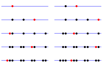
The following is en example when the irrational number is set to $\sqrt{5}$ .

The proof is surprisingly short:
First, one can show that for each function $f_k(x)=e^{2 \pi i k x}$ , where $i$ is the imaginary unit, $k = 0, 1, \cdots$ , we have
$\lim_{n \to \infty}\left(\frac{1}{n} \sum_{j=1}^n f_k(u_j)\right)= \lim_{n \to \infty}\left(\frac{1}{n}\sum_{j=1}^n e^{2 \pi i k u_j}\right) = 0$ : The nice thing is that $e^{2 \pi i k \{j \alpha\}}$ equals to $e^{2 \pi i k j \alpha}$ — the fractional operator $\{\cdot\}$ disappears because $e^{2 \pi i m}$ is 1 for any integer $m$ . Therefore, we can compute $\sum_{j=1}^n e^{2 \pi i \{j \alpha\}}$ easily, it is simply $\sum_{j=1}^n e^{2 \pi i k j \alpha}$ , which is nothing but a geometric sum $\sum_{j=1}^n (e^{2 \pi i k \alpha})^j$ , which is $((e^{2\pi i k \alpha})^{n+1}-e^{2\pi i k \alpha})/(e^{2\pi i k \alpha}-1)$ . Since $\alpha$ is irrational, $e^{2\pi i k \alpha}$ is never 1, hence the denominator is nonzero. The magnitude of $((e^{2\pi i k \alpha})^{n+1}-e^{2\pi i k \alpha})/(e^{2\pi i k \alpha}-1)$ is upper bounded by $2/\vert e^{2\pi i k \alpha}-1\vert$ , as the magnitude of $e^{2\pi i k \alpha}$ is 1. Therefore,
$\lim_{n \to \infty}\frac{1}{n}\sum_{j=1}^n f_k(u_j) \leq \lim_{n \to \infty} \frac{1}{n}\frac{2}{\vert e^{2\pi i k \alpha}-1\vert}=0$ .

Since $\int_{0}^1 f_k(x)dx = \int_{0}^1 e^{2 \pi i k x}dx=0$ , we have
$\lim_{n \to \infty}\frac{1}{n}\sum_{j=1}^n f_k(u_j) = \int_{0}^1 f_k(x)dx$ . In particular, this implies that for all trigonometric polynomials $f(x)=\sum_{k=0}^n (a_k \sin{2\pi k x} + b_k \cos{2 \pi k x})$ , where $a_k, b_k, k= 0, \cdots$ are real numbers, it holds that
$\lim_{n \to \infty} \frac{1}{n}\sum_{j=1}^n f(u_j) = \int_0^1 f(x)dx$ . Using Weierstrass’ approximation theorem, one can show that the equation holds for all functions $f_{[a,b)}(x)$ , where $f_{[a,b)}(x) = 1$ for $x \in [a,b)$ and 0 otherwise, $a, b \in [0,1]$ –this is precisely the requirement for $\{u_j\}_{j=1}^{\infty}$ being uniformly distributed over $[0,1]$ .

The Mathematica code to visualize $\{u_j\}_{j=1}^{\infty}$ :

pts = Table[
   Map[Point[{#, 0}] &, 
      FractionalPart /@ N[Table[i Sqrt[5], {i, 1, j}]]] /. {x___, 
       y_} :> {{PointSize[Large], x}, {PointSize[Large], Red, y}} // 
    Graphics, {j, 1, 10}];

unitinterval =
  Graphics[{Blue, Line[{{0, 0}, {1, 0}}]}, AspectRatio -> 1/4];

GraphicsGrid[Partition[Map[Show[unitinterval, #] &, pts], 2]]

e2718281828459045

Month: November, 2013

November 17, 2013

A short summary of interesting algorithm interview questions

November 16, 2013

Uniform distribution of infinite sequences

November 13, 2013

Kissing number problem