e2718281828459045

November 17, 2013

A short summary of interesting algorithm interview questions

These interviews questions are from multiple posts on mitbbs. I find them more interesting than “convert a linked list to a binary tree”-typed interview questions and straight forward questions such as “what is FFT?”, because these questions provide contexts — so they are more like real life problems than merely algorithm exercises.

1. Stock price smoothing, Gaussian smoothing, FFT (Source: Two Sigma?).
2. Influencer, variation of CLRS exerise 22.1-6 “universal sink” (Source: LinkedIn)
3. auto racer, variation of counting inversion (Source: Rocket Fuel)
4. generate random samples from a distribution, Huffman encoding (Source: Google, original article)
5. 2D rainwater trapping, variation of sweep line (Source: Google)

Leave a comment

November 16, 2013

Uniform distribution of infinite sequences

This is another gem from the book “Geometric Discrepancy: an Illustrated Guide” by Matousek.

A sequence $\{u_1, u_2,\cdots\}$ is uniformly distributed over $[0,1]$ if for each interval $[a,b) \subset [0,1]$ ,
$\lim_{n \to \infty}\frac{1}{n}\vert \{u_1, u_2,\cdots, u_n\}\cap [a,b) \vert = b-a$ . How does a uniformly distributed sequence over the unit interval look like?

The definition of uniformly distributed sequence is a very natural generalization of the problem of approximating uniform distribution in 1-dimension with finitely many points: suppose we want to place $n$ points uniformly over $[0,1]$ , the most natural approach is to place the $n$ points equidistantly over the unit interval. For a sequence of infinitely many numbers, we would like them to sweep “uniformly” over the interval. Note that for a fixed $n$ , if we randomly pick $n$ numbers randomly and uniformly from $[0,1]$ , the percentage of points falling in the interval $[a,b)$ is $b-a$ .

Weyl’s criterion is the following: for each irrational number $\alpha$ , the sequence $\{u_1, u_2,\cdots\}$ , where $u_n$ is the fractional part of $n \alpha$ , denoted by $\{n \alpha\}$ ( $\{x\}$ is the fractional part of $x$ ), is uniformly distributed over $[0,1]$ .

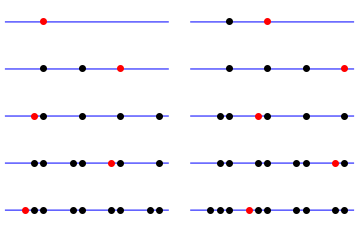
The following is en example when the irrational number is set to $\sqrt{5}$ .

The proof is surprisingly short:
First, one can show that for each function $f_k(x)=e^{2 \pi i k x}$ , where $i$ is the imaginary unit, $k = 0, 1, \cdots$ , we have
$\lim_{n \to \infty}\left(\frac{1}{n} \sum_{j=1}^n f_k(u_j)\right)= \lim_{n \to \infty}\left(\frac{1}{n}\sum_{j=1}^n e^{2 \pi i k u_j}\right) = 0$ : The nice thing is that $e^{2 \pi i k \{j \alpha\}}$ equals to $e^{2 \pi i k j \alpha}$ — the fractional operator $\{\cdot\}$ disappears because $e^{2 \pi i m}$ is 1 for any integer $m$ . Therefore, we can compute $\sum_{j=1}^n e^{2 \pi i \{j \alpha\}}$ easily, it is simply $\sum_{j=1}^n e^{2 \pi i k j \alpha}$ , which is nothing but a geometric sum $\sum_{j=1}^n (e^{2 \pi i k \alpha})^j$ , which is $((e^{2\pi i k \alpha})^{n+1}-e^{2\pi i k \alpha})/(e^{2\pi i k \alpha}-1)$ . Since $\alpha$ is irrational, $e^{2\pi i k \alpha}$ is never 1, hence the denominator is nonzero. The magnitude of $((e^{2\pi i k \alpha})^{n+1}-e^{2\pi i k \alpha})/(e^{2\pi i k \alpha}-1)$ is upper bounded by $2/\vert e^{2\pi i k \alpha}-1\vert$ , as the magnitude of $e^{2\pi i k \alpha}$ is 1. Therefore,
$\lim_{n \to \infty}\frac{1}{n}\sum_{j=1}^n f_k(u_j) \leq \lim_{n \to \infty} \frac{1}{n}\frac{2}{\vert e^{2\pi i k \alpha}-1\vert}=0$ .

Since $\int_{0}^1 f_k(x)dx = \int_{0}^1 e^{2 \pi i k x}dx=0$ , we have
$\lim_{n \to \infty}\frac{1}{n}\sum_{j=1}^n f_k(u_j) = \int_{0}^1 f_k(x)dx$ . In particular, this implies that for all trigonometric polynomials $f(x)=\sum_{k=0}^n (a_k \sin{2\pi k x} + b_k \cos{2 \pi k x})$ , where $a_k, b_k, k= 0, \cdots$ are real numbers, it holds that
$\lim_{n \to \infty} \frac{1}{n}\sum_{j=1}^n f(u_j) = \int_0^1 f(x)dx$ . Using Weierstrass’ approximation theorem, one can show that the equation holds for all functions $f_{[a,b)}(x)$ , where $f_{[a,b)}(x) = 1$ for $x \in [a,b)$ and 0 otherwise, $a, b \in [0,1]$ –this is precisely the requirement for $\{u_j\}_{j=1}^{\infty}$ being uniformly distributed over $[0,1]$ .

The Mathematica code to visualize $\{u_j\}_{j=1}^{\infty}$ :

pts = Table[
   Map[Point[{#, 0}] &, 
      FractionalPart /@ N[Table[i Sqrt[5], {i, 1, j}]]] /. {x___, 
       y_} :> {{PointSize[Large], x}, {PointSize[Large], Red, y}} // 
    Graphics, {j, 1, 10}];

unitinterval =
  Graphics[{Blue, Line[{{0, 0}, {1, 0}}]}, AspectRatio -> 1/4];

GraphicsGrid[Partition[Map[Show[unitinterval, #] &, pts], 2]]

Leave a comment

November 13, 2013

Kissing number problem

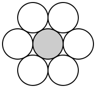
I was looking for an interesting topic for a 20-minute presentation yesterday and stumbled upon an interesting article: Kissing numbers, Sphere packings and Some unexpected proofs.

(Figure from wikipedia)

It has a similar flavor as the oddtown problem: an elegant application of basic linear algebra methods.

Leave a comment

October 27, 2013

Fun with TikZ

TikZ/PGF is a powerful and interesting tool to draw figures in latex. For example, one can draw “regular” objects like this in Tikz:

In principle anything that can be described mathematically can be drawn with TikZ (for example most geometric shapes such as circles, rectangles, etc.) relatively effortlessly. Here are two new examples drawing irregular objects in TikZ:

(1) Simulating hand-drawn lines with TikZ (link)

(2) Poppy flower (link)

Leave a comment

October 25, 2013

Discrepancy of corner rectangles

Given a set $P$ of $n$ points in a unit square in the plane $[0,1]^2$ , define the $L_2$ discrepancy for corners of $P$ as
$D_2(P, \mathcal{C}) = \sqrt{\int_{[0,1]^2}(D(P, C_x))^2dx}$ ,
where $C_x$ is the corner rectangle $[0,x_1) \times [0,x_2)$ for the point $x = (x_1,x_2) \in [0,1]^2$ , and $D(P,C_x)$ is a function of $x$ , which is defined as
$D(P,C_x) = n\cdot {\rm vol}(C_x)-\vert P \cap C_x\vert$ (the discrepancy of $P$ with respect to the corner rectangle $C_x$ ). $\mathcal{C}$ is the set of all corner rectangles $\{C_x \vert x \in [0,1]^2\}$ .

The discrepancy for corners of $P$ measures how close $P$ approximates a uniform distribution of $n$ points in the unit square: roughly speaking, if $P$ “truly” uniformly distributes over $[0,1]^2$ , then for an arbitrary corner rectangle $C_x$ , $x \in [0,1]^2$ , the expectation of the number of points falling in $C_x$ , which is $\vert P \cap C_x \vert$ , is $n \cdot {\rm vol}(C_x)$ . So the quantity $D(P, C_x)$ , which is the difference the the latter and the former, measures the deviation of $P$ from the uniform distribution witnessed by the corner rectangle $C_x$ .

One can ask (1) how well can we approximate the uniform distribution? That is, for each $n$ , we would like to have a configuration of $n$ points in $[0,1]^2$ such that $D_2(P, \mathcal{C})$ is small. For example, one candidate might be the grid $\sqrt{n} \times \sqrt{n}$ in the unit square (Although this seems to be a good way to put $n$ points into the unit square as “uniformly” as possible intuitively, there are more “uniform” candidates). (2) on the other hand, is it the case that no matter how we distribute the $n$ points, there is always a large gap between the approximation and the ideal uniform distribution? That is, for every $n$ -point set $P$ , the discrepancy is at least $f(n)$ for some function $f$ depending on $n$ ?

Both questions are the starting points of discrepancy theory. They both are hard questions, yet they have surprisingly elementary and elegant simple solutions. The following lower bound proof of $\Omega(\sqrt{\log n})$ of $D_2(P,\mathcal{C})$ is from “Geometric Discrepancy” by Matousek. The proof is quite short, but is indeed ingenious (it is that kind of proof that gives the feeling of “opening a magical door”).

Note that for a fixed point set $P$ , the function $D(P,C_x)$ , which will be denoted by $D(x)$ from now on (as we fix $P$ ), is not hard to compute: $D(x) = n \cdot {\rm vol}(C_x) - \vert P\cap C_x \vert = n x_1 x_2 - \vert P \cap C_x \vert$ , $x =(x_1,x_2)$ , is a piece-wise continuous function over the unit square. The second term, $\vert P \cap C_x \vert$ changes discretely as we move the anchor $x$ over $[0,1]^2$ to include (resp. exclude) new points of $P$ into (reap. from) the corner rectangle $C_x = [0,x_1)\times [0,x_2)$ . Indeed, it can be computed in $O(n(\log n)^2)$ time. However, the difficulty is that we need to take the lower bound $\inf_{P \subset [0,1]^2, \vert P \vert = n} D_2(P,\mathcal{C})$ . It is even quite unclear how the discrepancy changes as we vary $P$ , hence it seems rather hard to get hold of the quantity $\inf_P D(P,\mathcal{C})$ .

Roth’s proof uses a clever auxiliary function $F:[0,1]^2 \to \{-1,0,1\}$ to obtain the lower bound: we have
$\int_{[0,1]^2} F(x)D(x)dx \leq \sqrt{\int_{[0,1]^2}(F(x))^2 dx} \sqrt{\int_{[0,1]^2}(D(x))^2 dx}$ by Cauchy-Scharwz inequality. Then a lower bound of $D(P,\mathcal{C})$ is
$\sqrt{\int_{[0,1]^2} (D(x))^2 dx} \geq (\int_{[0,1]^2} F(x)D(x)dx)/(\sqrt{\int_{[0,1]^2}(F(x))^2 dx})$ . So if we could construct a function $F(\cdot)$ such that
(1) $\int_{[0,1]^2} F(x)D(x)dx$ is $\Omega(\log n)$ ;
(2) $\sqrt{\int_{[0,1]^2}(F(x))^2 dx}$ is $O(\sqrt{\log n})$ .
Then we get the desired lower bound. (The construction of $F(\cdot)$ is quite magical as it vaguely seems like some sort of amortization of the discrepancy, but I cannot find any intuitive explanation for it.)

Here is the construction:
Choose an integer $m$ such that $2n \leq 2^m < 4n$ . Define $m$ function $f_j: [0,1]^2 \to \{-1,0,1\}$ , $j = 0,\cdots, m$ , where $f_j$ is defined as following: partition the unit square into $2^j$ vertical slabs, then again partition it into $2^{m-j}$ horizontal slabs. So we get $2^m$ rectangles in total. If a rectangle $R$ contains any point from $P$ , then $f_j$ is 0 over $R$ ; otherwise, $R$ is free of points from $P$ , then we again partition $R$ into four quadrants (by cutting it from the middle vertically first, then horizontally second), and $f_j$ takes the value -1, +1, -1, +1 over the upper left, lower left, lower right, upper right sub-rectangles.

The remarkable properties of the family of functions $\{f_j\}_{j=0}^m$ are:
(1) $f_i$ and $f_j$ is orthogonal: that is, $\int_{[0,1]^2} f_i(x)f_j(x)dx = 0$ for $i \neq j$ . We set $F = \sum_{j=0}^m f_j$ . The orthogonality immediately implies that $\int_{[0,1]^2}(F(x))^2 dx$ is at most $m+1$ , which is $\Theta(\log n)$ .
(2) $\int_{[0,1]^2}f_j(x)D(x)dx$ is $\Omega(1)$ . This immediately implies that $\int_{[0,1]^2}F(x)D(x)dx$ is $\Omega(m)$ , which is $\Omega(\log n)$ .

Leave a comment

October 23, 2013

An example of recursive definition

Recursive data types are ubiquitous in functional programming language. Two common examples are trees and lists. Here is a nice and slightly different example from “The Little MLer”:

datatype
   slist = 
   Empty
  |Scons of (( sexp) * ( slist))
and 
   sexp =
   An_atom of 
  |A_slist of ( slist)

Here $\alpha$ is a type variable. For example, we can let $\alpha$ be fruit, where fruit is a data type defined as

datatype fruit =
  Apple
 |Pear

The slightly strange thing about $\alpha$ slist is when you try to describe the set of values for this data type: if we say “ $\alpha$ slist is a set, which contains an element Empty, and Scons of pairs of $\alpha$ sexp and $\alpha$ slist…”–but this definition does not make much sense as we have not defined $\alpha$ sexp yet. If we try to define $\alpha$ sexp, we run into the same problem: “ $\alpha$ sexp is a set, which contains elements An_atom(x), where $x$ is of type $\alpha$ , and A_slists of $\alpha$ slist”–we have not defined what $\alpha$ slist yet.

The way to get out of this logical dilemma is to use induction. For example, for the type fruit slist and fruit sexp, we define the two sets as following:
(1) $A_0 = \{{\rm Empty}\}$ , $B_0 = \{{\rm An\_atom(Apple)}, {\rm An\_atom(Pear)}\}$
(2) $A_{i+1} = \{{\rm Scons}(x,y)\vert x \in \cup_{j=0}^i A_i, y \in \cup_{j=0}^i B_i\}$ ,
$B_{i+1} = \{{\rm A\_slist}(x) \vert x \in \cup_{j=0}^i A_i\}$ , $i \geq 1$ .

Then the set of values for fruit slist (resp. fruit sexp) is $\cup_{i=0}^{\infty}A_i$ (resp. $\cup_{i=0}^{\infty}B_i$ ).

Leave a comment

October 19, 2013

Longest oscillating subsequence (zigzag sequence)

Longest oscillating subsequence: Given a sequence $A$ of distinct numbers $\{a_i\}_{i=1}^n$ , an oscillating subsequence is a subsequence $\{a_{i_j}\}_{j=1}^m$ , such that the sign of the difference between adjacent elements in $\{a_{i_j}\}_{j=1}^m$ alternates. The goal is to find a longest such subsequence.

For example, given a sequence 9,12,1,7,3,6,8,4, a longest oscillating subsequence is 9,12,1,7,3,8,4. The following is a linear time greedy algorithm. The algorithm is from here. We can break the sequence $A$ into monotone runs: a consecutive subsequence $a_i, a_{i+1},\cdots, a_{i+(j-1)}$ is a monotone run of $A$ if (1) the length of the subsequence, $j$ , is at least 2; (2) the sign of adjacent elements in this subsequence does not change; (3) the subsequence $a_i,\cdots, a_{i+(j-1)}$ is maximal in the sense that no other monotone run of $A$ strictly contains it. In other words, it is not possible to extend this subsequence either to the left or to the right (either because we reach the end of the sequence $A$ , or because the sign between adjacent elements changes). The longest oscillating subsequence is formed by the first element from each monotone run and the last element of the last monotone run. To see why this is true, note that any oscillating subsequence contains at most two elements from 2 consecutive monotone runs, except the last monotone run. That is, suppose we have monotone runs $M_1, M_2, \cdots, M_k$ , then any oscillating subsequence contains at most two elements from $M_1$ and $M_2$ , and at most two elements from $M_2$ and $M_3$ , and so on. So we can prove that the length of such a sequence is $k+1$ by induction.

It is easy to see that the algorithm is linear since each adjacent monotone runs overlap at exactly one element: so for each $a_i$ , either we extend the current monotone run, or we start a new monotone run.

The Haskell code for this greedy algorithm:

monotone :: ([Int], [Int]) -> (Int->Int->Bool)-> ([Int], [Int])
monotone (x, []) _ = (x, [])
monotone ([], x:xs) f = monotone ([x], xs) f
monotone (x, ally@(y:ys)) f
    |f (last x) y = monotone (x ++ [y], ys) f
    |otherwise = (x, last x : ally)

monotone' :: [Int] -> (Int->Int->Bool) -> ([Int], [Int])
monotone' x f = monotone ([], x) f

greedyzigzag :: [Int] -> [Int]
greedyzigzag [] = []
greedyzigzag [x] = [x]
greedyzigzag [x,y] = [x,y]
greedyzigzag all@(x:y:ys) = let (firstrun, rest) = monotone' all f
                                f = if x < y then (<) else (>)
                            in if (rest == []) then [head firstrun, last firstrun] else head firstrun:greedyzigzag rest

greedyzigzag' :: [Int] -> Int
greedyzigzag' = length.greedyzigzag

This is the quadratic algorithm, modified from the getSnake code from the previous post which computes the longest zig sequence and longest zag sequence separately:

longest :: [Int] -> Int -> (Int->Int->Bool, Int->Int->Bool) -> [Int]
longest [x] y (f,_)
    |f x y = [x]
    |otherwise = []

longest (x:xs) y (f,g)
    |g x y = longest xs y (f,g)
    |otherwise =
        let startwithx = x : (longest xs x (g,f))
            notwithx = longest xs y (f, g)
            len1 = length startwithx
            len2 = length notwithx
        in if len1 > len2 then startwithx else notwithx

longestzig :: [Int] -> [Int]
longestzig x = longest x (length x) ((<),(>))

longestzig' :: [Int] -> Int -> [Int]
longestzig' x y = longest x y ((<),(>))

longestzag :: [Int] -> [Int]
longestzag x = longest x 0 ((>), (<))

longestzag' :: [Int] -> [Int]
longestzag' x y = longest x y ((>), (<))

longestzigzag' :: [Int]->Int
longestzigzag' x = maximum $ map (length.($x)) [longestzig, longestzag]

Leave a comment

October 19, 2013

Clubs in oddtown

Oddtown has 32 inhabitants. They would like to form clubs, following the “oddtown” rules:
(1) Each club has an odd numbers of members;
(2) The number of common members between any two distinct clubs is even.
The question is what is the largest number of clubs they can form?

As a trivial example, suppose the town has only two inhabitants ${1,2}$ . They can form two clubs: $C_1 = \{1\}$ and $C_2 = \{2\}$ . In fact, that is the largest number of clubs they can form (because the other two sets, $\emptyset$ and $\{1,2\}$ are not valid clubs since their cardinality is even).

It is easy to see that for Oddtown, they can form 32 clubs, for example, $C_{i} = \{i\}$ , $i = 1,\cdots, 32$ is a valid set of clubs. The question is that whether 32 is the largest number of clubs they can form? The problem has a surprisingly simple and elegant solution (using linear algebra method).

The question, and the following solution, are from “Linear algebra methods in combinatorics with applications to geometry and computer science” by L.Babai and P.Frankl.

Consider each club as a vector in $\mathbb{F}_2^{32}$ , where $\mathbb{F}_2$ is the field $\mathbb{Z}/2\mathbb{Z}$ (the field of $\{0,1\}$ ): represent club $C_i \subset \{1,\cdots, 32\}$ as a vector $v_i$ , where the $j^{\rm th}$ entry is 1 if $j$ is a member of club $C_i$ , and 0 otherwise. Note that the inner product $v_i$ and $v_j$ , $v_i \cdot v_j$ , is the number of common members between $C_i$ and $C_j$ modulo 2. From rule (1), $v_i \cdot v_i = 1$ , since it is the cardinality of $C_i$ , is an odd number, modulo 2; from rule (2), $v_i \cdot v_j = 0$ , $j \neq i$ , since it is an even number modulo 2. The key observation is that the set of vectors is linearly independent over $\mathbb{F}_2$ . Suppose there are $m$ clubs, $C_1,\cdots, C_m$ , and thus respectively $m$ vectors $v_1, \cdots, v_m$ . It suffices to show that if
$a_1 v_1 + a_2 v_2 + \cdots + a_m v_m = 0$ (*), where each $a_i \in \mathbb{F}_2$ , then $a_i = 0$ for all $i =1,\cdots,m$ .

Consider the equation
$a_1 v_1 \cdot v_1 + a_2 v_2 \cdot v_1 + \cdots + a_m v_m \cdot v_1 = 0$ .
Since $v_1 \cdot v_1$ is 1, and each $v_j \cdot v_1$ , $j \neq 1$ is 0, $a_1$ therefore must be 0. Following similar approach, we conclude that $a_i$ is 0 for each $1 \leq i \leq m$ . Hence the set $m$ vectors is linearly independent — which implies that $m$ is at most 32.

Leave a comment

October 14, 2013

A curious application of recurrence

Express $(\sqrt{2} + \sqrt{3})^{1980}$ as a decimal fraction, what are the digits immediately to the left and to the right of the decimal point?

For example, for $(\sqrt{2} + \sqrt{3})^2 = 5 + 2\sqrt{6} \approx 9.89$ , the digit immediately to the left of the decimal point is 9, and the digit to the right is 8.

This problem, and the following proof is from the book “Discrete Mathematics” by Martin Aigner.

The problem and the proof are both quite nice, because at first sight this problem seems have nothing to do with recurrence.

Here is the sketch of the proof: first observe that $(\sqrt{2}+\sqrt{3})^{2n}$ , $n \in \mathbb{N}$ is the sum of an integer and a multiple of $\sqrt{6}$ . For example, for $n = 1$ , $(\sqrt{2}+\sqrt{3})^2 = 5 + 2\sqrt{6}$ . This is straight forward from binomial theorem:
$(\sqrt{2}+\sqrt{3})^{2n} = \sum_{k=0}^{2n} {2n \choose k}(\sqrt{2})^{2n-k}(\sqrt{3})^k$ .
For $k$ odd, a term $(\sqrt{2})^{2n-k}\sqrt{3}^k$ is a multiple of $\sqrt{6}$ ; for $k$ even, this term is an integer. So the above expression is a summation of alternating integers and (integral) multiples of $\sqrt{6}$ , therefore, we have
$(\sqrt{2}+\sqrt{3})^{2n} = a_n + b_n \sqrt{6}$ , for $n = 0, 1, \cdots$ , where $a_n, b_n$ are integers.

The recurrence formula for $a_n$ and $b_n$ is:
$a_{n+1} = 5a_n + 12 b_n$ , $b_{n+1} = 2a_n + 5 b_n$ . Using the machinery of generating functions, we get a closed form of $a_n$ as
$a_n = \frac{1}{2}\left((5+2\sqrt{6})^n+(5-2\sqrt{6})^n\right)$ . As $(\sqrt{2}+\sqrt{3})^{2n} = (5+2\sqrt{6})^n$ , we get $a_n = \frac{1}{2}(a_n + b_n\sqrt{6}+(5-2\sqrt{6})^n)$ , which implies that
$a_n = b_n \sqrt{6} + (5-2\sqrt{6})^n$ . (*)

Note that the fractional part of $(\sqrt{2}+\sqrt{3})^{2n} = a_n + b_n\sqrt{6}$ is the fractional part of $b_n \sqrt{6}$ . From (*), what can we infer about $b_n \sqrt{6}$ ? Because $a_n$ is an integer, the fractional part of $b_n \sqrt{6}$ and the fractional part of $(5-2\sqrt{6})^n$ must sum up to an integer. The crucial observation is that $5 - 2\sqrt{6} < 1$ , therefore, when it is raised to a large power, say, 990, $(5-2\sqrt{6})^{990}$ is very close to 0 — it is of the form "0.000….". This implies that $b_n \sqrt{6}$ , where $n = 990$ must be of the form "0.999…..". Thus, the digit immediately to the right of the decimal point in $(\sqrt{2}+\sqrt{3})^{2n}$ , $n = 990$ , is 9.

To determine the digit immediately to the left of the decimal point in $(\sqrt{2}+\sqrt{3})^{2n}$ , $n = 990$ , note that it is determined by $a_{990}$ and the integral part of $b_{990}\sqrt{6}$ . Following a similar reasoning as the above, we see that the integral part of $b_{990}\sqrt{6}$ is one less than $a_{990}$ (which is an integer, of course) modulo 10. Therefore, the last digit of the integral part of $(\sqrt{2}+\sqrt{3})^{1980}$ is completely determined by $a_{990}$ : to be precise, it is $2a_{990} - 1$ modulo 10. For $n = 0, 1, \cdots, 5$ , the first 6 pairs of the last digits of $(a_i, b_i)$ is $(1, 0), (5, 2), (9, 0), (5, 8), (1, 0), (5, 2)$ . Therefore, it is periodic with period 4. Hence, $a_{990}$ is 9 as $990 \equiv 2 \mod 4$ . Therefore, the digit immediately to the left of the decimal point of $(\sqrt{2}+\sqrt{3})^{1980}$ is $2 \times 9 - 1 \equiv 7 \mod 10$ .

Leave a comment

October 10, 2013

Zigzag sequence

Given a sequence of distinct numbers $\{a_i\}_{i=1}^n$ , the sequence is a zig-zag sequence if either (1) $n \leq 1$ , that is, an empty sequence or a sequence with a single element are both the trivial zig-zag sequence; or (2) otherwise, the sign of the difference between adjacent element alternates.

For example, the sequence 2,3,1 is a zig-zag sequence because 2 < 3 and 3 > 1 while 1,2,3 is not. The questions are
(1) given a sequence of numbers, compute a zigzag sequence of these numbers;
(2) given $n$ , count the number of zigzag sequences of $[n]$ ( $[n]$ denotes the set of elements $1, 2, \cdots, n$ ).

The first question is easy and it has a linear time algorithm: if the input has only 1 element, we are done. So suppose the input has at least two elements. Scan the sequence from left to right, for two adjacent element $a_i$ and $a_{i+1}$ , $1 \leq i < n$ , if they satisfy the inequality (which is “>” for $i$ even and “<” for $n$ odd), then increment $i$ ; otherwise, swap $a_i$ and $a_{i+1}$ . Then increment $i$ . We repeat this until we reach $i = n-1$ ..

As an example, consider the input 4, 1, 2, 3, 5: the target is to get a sequence $a_1 < a_2 > a_3 < a_4 > a_5$ . Let’s number the elements, so $a_1 = 4$ , $a_2 = 1$ , and so on.

The starting sequence is $4, 1, 2, 3, 5$ .
$i = 1$ :
Since 4 > 1, we swap 4 and 1, the new sequence is 1, 4, 2, 3, 5;

$i = 2$ :
Since 4 > 2, it satisfies that $a_2 > a_3$ .

$i = 3$ :
Since 2 < 3, it satisfies that $a_3 < a_4$ .

$i = 4$ :
Since 3 < 5, we swap 5 and 3, to get 1, 4, 2, 5, 3.

The output is hence 1, 4, 2, 5, 3.

The recursive algorithm does not differ too much from the above imperative one.
A sequence $A[1..n]$ is a “happy zigzag” sequence if either (1) $n \leq 1$ , in which case it is a trivial happy zigzag sequence; or (2) $n \geq 2$ , $A[1] < A[2]$ , and $A[2..n]$ is a sag zigzag sequence.
A sequence $A[1..n]$ is a “sad zigzag” sequence if either (1) $n \leq 1$ , in which case it is a trivial sad zigzag sequence; or (2) $n \geq 2$ , $A[1] > A[2]$ , and $A[2..n]$ is a happy zigzag sequence.
To compute a happy zigzag sequence, if the first two elements of $A[1..n]$ satisfies $A[1]<A[2]$ , then we compute a sad zigzag sequence of $A[2..n]$ , and the output is $A[1]$ concatenated with this sequence; otherwise, we swap $A[1]$ and $A[2]$ , then proceed as the previous case.

getSnake :: (Ord a) => [a] -> (a->a->Bool, a->a->Bool) -> [a]
getSnake [] _ = []
getSnake [x] _ = [x]
getSnake (x:y:xs) (f,g)
    |f x y = x : (getSnake (y:xs) (g,f))
    |otherwise = y : (getSnake (x:xs) (g,f))

getSnake' :: (Ord a) => [a] -> [a]
getSnake' x = getSnake x ((<), (>))

The second problem is much harder than the first one. The number of zig-zag sequences for $n = 1$ to 7 are 1,2,5,16,61,272,1385. Look familiar? Here is the surprising connection from [1]:
$\tan x = \frac{x}{1!} + \frac{2x^3}{3!} + \frac{16 x^5}{5!} + \frac{272 x^7}{7!} + \cdots$
$\sec x = \frac{1 x^0}{0!} + \frac{1x^2}{2!} + \frac{5x^4}{4!} +\frac{61x^6}{6!} +\cdots$ .

An interesting object is the following zigzag triangle from [1]:

         1 
        0 1
       1 1 0
     0  1  2 2
   5  5  4  2  0
  0  5 10 14 16 16
61 61 56 46 32 16 0

The triangle is filled in the following way: the first row is 1. The $i^{\rm th}$ row is computed from the $(i-1)^{\rm th}$ row: we alternate the direction of filling up the row, and the starting element is 0. We fill up the row using the zig-zag rule:

  a
b -> (a+b)

The key observation is that the $i^{\rm th}$ element in $n^{\rm th}$ row is the number of zigzag sequence ending with $i$ : for example, for $n = 5$ , the zigzag sequences are the following (sorted by ending element):
[[3,4,2,5,1],[2,5,3,4,1],[3,5,2,4,1],[2,4,3,5,1],[4,5,2,3,1],[1,4,3,5,2],[4,5,1,3,2],[1,5,3,4,2],[3,5,1,4,2],[3,4,1,5,2],[1,4,2,5,3],[1,5,2,4,3],[2,5,1,4,3],[2,4,1,5,3],[2,3,1,5,4],[1,3,2,5,4]]
The fifth row in the zigzag triangle is 5, 5, 4, 2, 0. This connection also gives an efficient recursive algorithm to count the number of zigzag sequences.

Update:
(1) The zigzag sequence is essentially alternating permutation.
(2) The recursive algorithm (getSnake) above can also be used to find a longest alternating permutation in quadratic time.

Reference
[1] Some Very Interesting Sequences, John H. Conway and Tim Hsu. (link)

Leave a comment